• Quantitative Tightening, as envisaged by the Fed, implies an equivalent, and ultimately sizeable, reduction of bank reserves on the liability side of the Fed’s balance sheet. 
• However, changes in monetary aggregates have little impact on the real economy or inflation. As a result, the money multiplier is simply likely to rise, as will the velocity of money.
• The most important effect of QT will be through long-term rates. Maturing UST’s will be replaced by new issues to the market. Once they reach their target pace, roll-offs will be equivalent to a full 60% of current net issuance.
• The effect will be moderate at first, but could be amplified by the knock-on effects on other asset prices, simultaneous policy changes by other central banks or a widening US federal deficit.

Balance Sheet Shift

The balance sheet reduction announced by the Federal Reserve will be a momentous event once it starts to unfold, unwinding the boldest policy experiment in the Fed’s history and bringing an eight-year old policy to a close. Yet, there are many misconceptions surrounding the role of monetary aggregates in the economy and the effects the balance sheet wind-down will have. What can be certain is that QT (Quantitative Tightening) will not simply be QE in reverse.  In what follows, we provide a brief explanation of how this will take place in practice and how it works itself through the economy.

To explore these issues, consider the actual simplified balance sheet of the Fed as of the end of July, which shows the outsized role of Treasury and MBS holdings on the asset side as well as the large bank reserve position on the liability side. Also worth noting is the temporarily small size of the government account (officially known as the TGA = Treasury General Account) as the Treasury runs down its funds until the debt ceiling is raised again.

Chart 1: Simplified Fed Balance Sheet, end-Jul 2017
In US$ billions

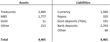
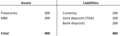
The TGA functions as the bank account of the Treasury, making the Fed the government’s ‘house bank’. Any transaction the Treasury undertakes (be it a payment to suppliers, for salaries or to collect taxes) passes via this account. Next, consider a stylized balance sheet as in chart 2:

Chart 2: Stylized Balance Sheet at t=0



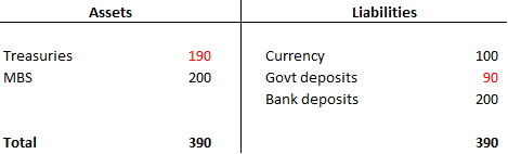
When a government debt security falls due, the Treasury pays the par amount to the Fed: in the first instance, its account gets debited by the amount due (e.g. $10 mn) and the asset side of the Fed balance sheet shrinks by the same amount as in chart 3.

Chart 3: Stylized Balance Sheet at t+1

The government’s cash position has now fallen, but it will want to maintain a reasonable amount of ‘petty cash’ in its account; the Treasury signalled that about a week worth of outflows (ca $300 mn) would be adequate, while others have argued for $500 mn or even as much as $1 trn (Ben Bernanke). [1]

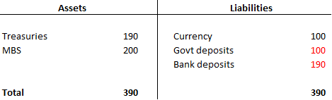
To this effect, the Treasury issues a new security and places its proceeds in the account. This time it is not the Fed that absorbs the issuance (so the asset side remains unaffected), but market participants. Whoever buys the security will ultimately debit a bank account and the bank will see its reserve account debited. The Treasury security is now no longer on the central bank’s balance sheet but held in the market. The Fed balance sheet is reduced and bank reserves are diminished.

Chart 4: Stylized Balance Sheet at t+2

The Money Multiplier: On a Rollercoaster

Armed with this understanding (that maturing of Treasuries held by the Fed cause bank reserves to decline even as the aggregate amount of Treasuries remains unchanged), we can ask how this might be contractionary or tighten financial conditions. A priori, one might expect bank lending or deposit growth to be directly affected by changes in bank reserves. After all, this was the case before the age of deregulation when required reserves represented a binding constraint on banking activities. The relationship between the monetary base (cash + bank reserves) and broad money (M1 or M2) – the money multiplier – was fairly stable back then.  Yet, the once stable money multiplier declined throughout the 1990s as financial markets were deregulated and more dramatically since 2009, with the advent of quantitative easing.

Chart 5: Money Multipliers

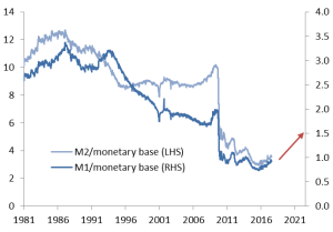
The recent decline reflects the sharp increase in bank reserves (the denominator of the money multiplier) without a concomitant increase in lending or deposits (numerator).[2] This is the Fed “pushing on a string”. If the money multiplier were constant one could expect falling bank reserves to provoke a reduction in broad money. But this is unlikely. Rather than cause economic adjustments, the money multiplier is simply a reflection of  underlying economic developments. As a result, it is simply likely to rise as the denominator shrinks and deposit growth continues to respond to the usual economic forces (perhaps rising as interest rates increase).

Bottom line: The money multiplier varies over time as there is no stable relationship between narrow and broad monetary aggregates. 

The Velocity of Money: Poor Policy Predictor

Nevertheless, there is concern among some market participants that the Fed’s balance sheet reduction would hamper broad money growth and would in turn put downward pressure on inflation. The theoretical foundation for this reasoning stems from the Quantity Theory of Money which postulates that M*V = P*Q (where M is the supply of money, V its velocity, P the price level and Q real output). In other words velocity V = PQ/M (i.e. nominal output divided by money). If V is stable and real output is determined by other,  non-monetary forces, this implies that prices vary in proportion to changes in the money supply .

Chart 6: Changes in Money Supply & Inflation, % yoy

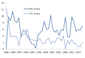
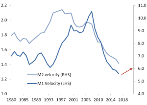
However, the empirical evidence does not bear this out: indeed, there is no stable relationship between money growth and inflation (Chart 6). In other words, the velocity of money is not stable (Chart 7). Looking ahead, the velocity of money of money will likely continue to be driven by economic fundamentals: with a tenuous link between money (M) and prices (P), the velocity will be determined by real output (Q). Just as V dropped when activity subsided in the wake of the financial crisis, it is likely to pick up as demand recovers and as will, eventually, prices. But it will be a corollary to fundamental developments, not a driver.

Chart 7: Velocity of Money (V=PQ/M)

Where Does This Leave Monetary Policy?

We have seen that: 1) lower Fed asset holdings imply lower bank reserves but that 2) there is no stable relationship between narrow and broad measures of money and that 3) there is no stable relationship between broad money and inflation. Does that mean that monetary policy is completely impotent and that the Fed’s asset sales will have no economic effect?

To gauge the direct effect of asset disposals, take a quick look at the size of the US Treasury market. The total value of Treasuries outstanding amounts to almost $16 trn (= 84% of GDP). [i] A large part of this is refinanced continually. Current gross issuance of Treasuries to the market is on average $700 bn per month or $8.4 trn per year. The majority of this serves to pay off debt coming due and as a result, net new issuance is just $50 bn per month or $600 bn per year. This corresponds closely to the size of the annual federal budget deficit. In other words, the fiscal deficit is almost entirely debt-financed.

Now consider QT. The Fed has announced that it would start the process by letting Treasuries roll off its balance sheet at a pace of $6 bn  per month (plus $4 bn of MBS). This would increase to a cap of $30 bn per month ($20 bn for MBS) or $360 bn per year. In terms of net additional Treasury supply, this is equivalent to a 60% increase in the federal deficit.

What effect would this have on yields? Successive rounds of QE were said to have lowered 10yr yields by some 75-100bps according to various studies. But the Fed does not plan to sell its securities outright and the roll-off will be at a fraction of the pace at which it purchased Treasuries during successive rounds of QE between 2008 and 2014. The balance sheet reduction will thus be much more gradual than the original build-up. In practice, the caps may not always be binding, especially outside the typical funding months (Feb, May, Aug, Nov). Indeed, JP Morgan estimate that only some $213 bn Treasuries come due in 2018 and some $264 bn in 2019. The impact will likely be spread unevenly across the curve. JP Morgan conservatively estimate that 2yr yields would rise by 7.3bps and 10yr yields by 25bps as a result of the additional supply.

But a 60% increase in net funding needs (assuming no change in the federal deficit) could nevertheless have a material impact. Here is why:

1. The above estimates may simply underestimate the ultimate effect on yields: ending the Fed’s QE experiment holds a bigger psychological portent for the market than a simple increase in Treasury supply.
2. The effect of the roll-offs could be amplified by similar shifts from other central banks. The ECB is likely to continue to scale back its asset purchases and the BoJ has also slowed the pace of purchases since adopting a yield target. As a result, German 10 yr Bund yields have already risen from negative in Q3 2016 to 0.4% recently and 10yr JGBs have gone from -5bps to +5bps over the same period.
3. A sell-off of fixed income securities could generate knock-on effects to other asset prices and trigger a self-reinforcing cycle. This in turn, could generate a much greater headwind for the economy than the direct interest rate effect alone.
4. Finally, the likely expansion of the federal deficit could amplify the effect of QT on yields, rather than simply be additive. The CBO recently raised its deficit estimate by $134 bn (to $693 bn) for 2017 and by $75 bn (to $563 bn) for 2018. This is on the basis of current legislation, without considering the effects of possible tax cuts or spending increases.

In sum, the Fed’s balance sheet reduction will create a new precedent for monetary policy in the US. A corollary is that bank reserves will shrink, money multipliers will rise and the velocity of money will likely accelerate. None of this will affect the economy much. These developments are simply the arithmetic equivalent of changes in policy. The most material impact on the economy will be through the effect on yields, given the additional net supply of Treasuries the policy will necessitate. This effect could be amplified through simultaneous policy changes elsewhere, spill-over effects into other markets and a widening US federal deficit.

[1] So far, the average balance over the past five years has been $150 mn but with huge monthly variations and higher balances lately.

[2] The money multiplier is defined as M1/monetary base or M2/monetary base. In a constrained system the multiplier equals 1/RR where RR stands for reserve requirement.

[i] Total US public debt is currently $19.8 trn (including intra-governmental debt), equivalent to 104% of GDP